Jekyll2024-05-27T21:10:09-03:00http://carlosgrohmann.com/feed.xmlProf. Carlos H. GrohmannPersonal website of Prof. Carlos H. Grohmann (IEE-USP, Brazil)
O que é um Invited Review?2020-08-23T00:00:00-03:002020-08-23T00:00:00-03:00http://carlosgrohmann.com/2020/08/23/bjgeo-review-papersUltimamente recebemos no Brazilian Journal of Geology (BJGEO) alguns pedidos de autores interessados em enviar artigos de revisão, os “Invited Reviews”. Mas o que é esse tipo de artigo? Uma revisão bibliográfica de tese pode ser publicada dessa maneira? Vamos ver:
O BJGEO prevê, em seu escopo, a publicação de artigos de revisão. Esses artigos podem ser solicitados pelos editores, mas especialistas reconhecidos também podem enviar espontaneamente artigos de revisão em seu campo de especialização. Mas nesse caso os autores devem entrar em contato com os editores para verificar seu interesse antes de enviar o artigo. E o processo de revisão por pares dos artigos de revisão segue os procedimentos usuais da revista.
Os artigos de revisão devem cobrir temas que sejam de interesse mais do que local, com alcance internacional e dirigidos a um público amplo. Espera-se que os autores tenham atuação e experiência prévia no tema, de modo a oferecer seu conhecimento e revisão de artigos prévios de sua autoria nos artigos de revisão. Dessa forma, artigos baseados essencialmente em revisões bibliográficas não são aceitos.
Um pequeno número de artigos de revisão já foi solicitado pelos editores a especialistas do Brasil e do exterior. Considerando-se o volume atual de submissões de artigos regulares, a expectativa dos editores é a de publicar até dois ou excepcionalmente três artigos de revisão por ano.
post by Carlos H. Grohmann
]]>C.H. GrohmannUTM 23S??2020-01-28T00:00:00-03:002020-01-28T00:00:00-03:00http://carlosgrohmann.com/2020/01/28/utm_southIf there’s one thing that I see all the time as a reviewer, is a map of some study area in Brazil with a caption like “UTM coordinates zone 23S”.
Don’t do that.
Why? I’ll tell you.
The UTM system divides the Earth into 60 zones (or fuses) of 6° longitude (plus some special zones at high latitudes). Zone 1 starts at 180° and zone numbering increases eastwards.
Then each zone is divided into 8° latitude bands, which are labeled by letters, starting with “C” at 80°S and going trhough the English alphabet until “X” (“I” and “O” are excluded because they are too similar to numbers 1 and zero).
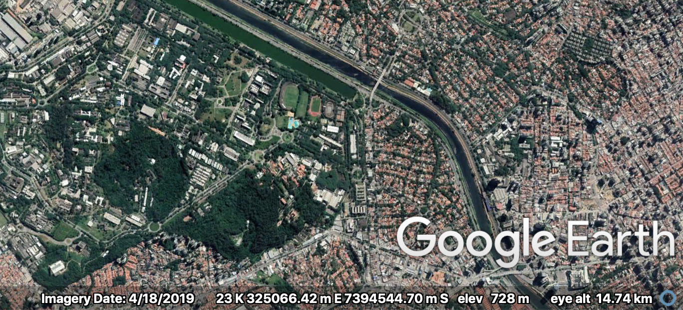
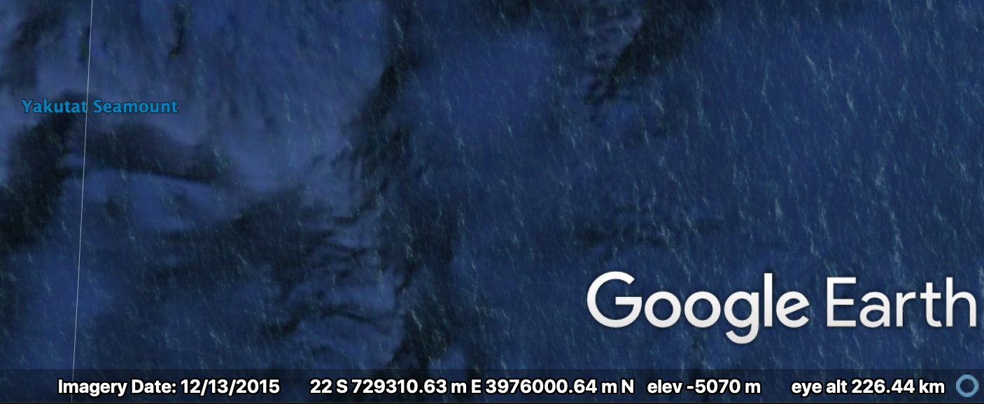
From that image we can see that a study area located in southeastern Brazil, like the city of São Paulo, will be in UTM zone 23K or 23J, but not 23S. Zone 23S is in the North Atlantic Ocean!
So why this happens at all? Simple, GIS software just don’t care! For a computer, all that matters is if your area is north or south of the Equator line. So a map projected in UTM, zone 23, southern hemisphere is just “23S”. And the same zone in the northern hemisphere is “23N”.
And what should I use in my maps?, you might ask. The right zone. Use “23K” or “23 south” but if you’re not studying the Yakutat Seamount, please don’t use “23S”.
And how can I find the right zone?, you might also ask? One simple trick is to use Google Earth. Just go to the software’s Preferences and in the coordinate system (in mine it says “Show Lat/Long”) you choose “Universal Tranverse Mercator”. Now the status bar at the bottom of the window will show you the coordinate and the UTM zone.
A little bit of São Paulo city, UTM zone 23K (screen capture from Google Earth)
Not São Paulo city, UTM zone 23S (screen capture from Google Earth)
post by Carlos H. Grohmann
]]>C.H. GrohmannFAQ about BJGEO2020-01-27T00:00:00-03:002020-01-27T00:00:00-03:00http://carlosgrohmann.com/2020/01/27/faq_bjgeoThe Brazilian Journal of Geology is the official publication of the Brazilian Geological Society. As the Deputy Editor, I receive emails with common questions about the journal. So I decided to crate a page with some useful information for potential authors.
Did your questions were answered in the FAQ? If not, leave a comment below.
post by Carlos H. Grohmann
]]>C.H. GrohmannTutorial - São Paulo City LiDAR2019-11-25T00:00:00-03:002019-11-25T00:00:00-03:00http://carlosgrohmann.com/2019/11/25/pmsp_lazThe São Paulo City Hall has just released free LiDAR data covering the city on their digital mapping platform, GeoSampa.
Also, just a few hours after the post went live, it received a comment from Fernando Gomes, who works at GEOINFO (the group maintaining GeoSampa) and shared a GitHub repository with a preliminary approach to analyze LiDAR data with Python and PDAL: https://github.com/geoinfo-smdu/usando-MDT. Nice!
Hope it helps. Spread the word!
]]>C.H. GrohmannNew site layout2019-02-03T00:00:00-02:002019-02-03T00:00:00-02:00http://carlosgrohmann.com/2019/02/03/new-layoutIf you are reading this it means my website is… alive and well! And you can see that this website has changed a bit. It loads faster, the visual is different (cleaner, I hope) and it works on all screen sizes (well, maybe not on a Nokia 3310).
The reason for all these wonderful features? Jekyll.
Jekyll is a Static Site Generator (SSG), meaning you create your content in simple text files using a markup language like markdown, and Jekyll converts it to a HTML/CSS static web page. That simple. No need for databases or complex stuff.
I found out about Jekyll when I decided to create the website for my Lab, the SPAMLab. That website is a Github page, hosted directly from our GitHub repository and build automatically every time you commit changes to the repository.
I bought my domain with namecheap.com, and they have a nice support page explaining how to serve your website through github pages. In this way, I can easily make the changes I want, commit only once (to github) and have my website both at carlosgrohmann.com and at carlosgrohmann.github.io.
]]>CarlosGrohmannThe SPAMLab has a website (and a blog)2018-04-27T00:00:00-03:002018-04-27T00:00:00-03:00http://carlosgrohmann.com/2018/04/27/the-spamlab-has-a-website-and-a-blogYes, that’s right. I finally managed to get the SPAMLab website up and running. It’s hosted on Github Pages: SPAMLab.github.io I’ll try to keep it updated with our research projects and activities. Stay tuned, and follow us on Twitter (@spamlab.iee) and Instagram (@spamlab.iee).]]>CarlosGrohmannPublish anything with us (just need to pay 1200 Euros)2017-05-24T00:00:00-03:002017-05-24T00:00:00-03:00http://carlosgrohmann.com/2017/05/24/publish-anything-with-us-just-need-to-pay-1200-eurosSo I just got this email:
Dear Dr. Grohmann, This is a follow up email regarding your invitation to write a chapter for a new Open Access book on “Multidimensional Flow Cytometry Techniques for Novel Highly Informative Assays,” edited by Dr. Marica Gemei. With over 2,800 titles published and a network that includes more than 98,000 international scientists and researchers, InTechOpen is a proven leader in Open Access book publishing. Your research will be available on the strongest Open Access book platform offering increased visibility and scientific impact. For complete project details visit: http://www.intechopen.com/welcome/668e45256b86d49c04db950772472e15/[my-email-was-here] If you are interested in publishing your research with us, submit a 1 page outline of your proposed chapter by 31 May, 2017 Please note that a payment of an Article Processing Charge of 1200 EUR will be required for all accepted chapters. This fee covers the costs associated with production and ensures that your chapter will be available online to read, share and download, for free. Let me know if you are interested in participating. I am available to answer any questions or discuss the possibility of an extension. Looking forward to hearing from you soon. Cordially, Teo Kos, from InTechOpen Publishing Process Manager ____________ InTech - open science | open minds Email: kos@intechopen.com Website: http://www.intechopen.com/ Phone: +385 (51) 770 447 Fax: +385 51 686166 Janeza Trdine 9 51000 Rijeka, Croatia
Easy, right? A little context: I’m a geologist, and I work with GIS, Remote Sensing and Digital Terrain Models. I had to look Wikipedia to see what flow cytometry is…
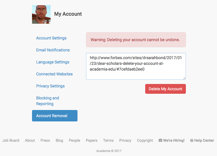
]]>CarlosGrohmannI deleted my account at Academia.edu2017-01-25T00:00:00-02:002017-01-25T00:00:00-02:00http://carlosgrohmann.com/2017/01/25/i-deleted-my-account-at-academia-eduI decided to delete my account at Academia.edu after reading Sarah Bond’s article in Forbes and Ethan Gruber’s post.
I’m thinking about hosting the PDFs of my papers and other documents with Zenodo or figshare (I already have some docs there).
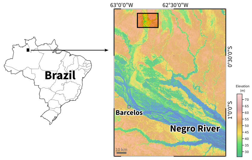
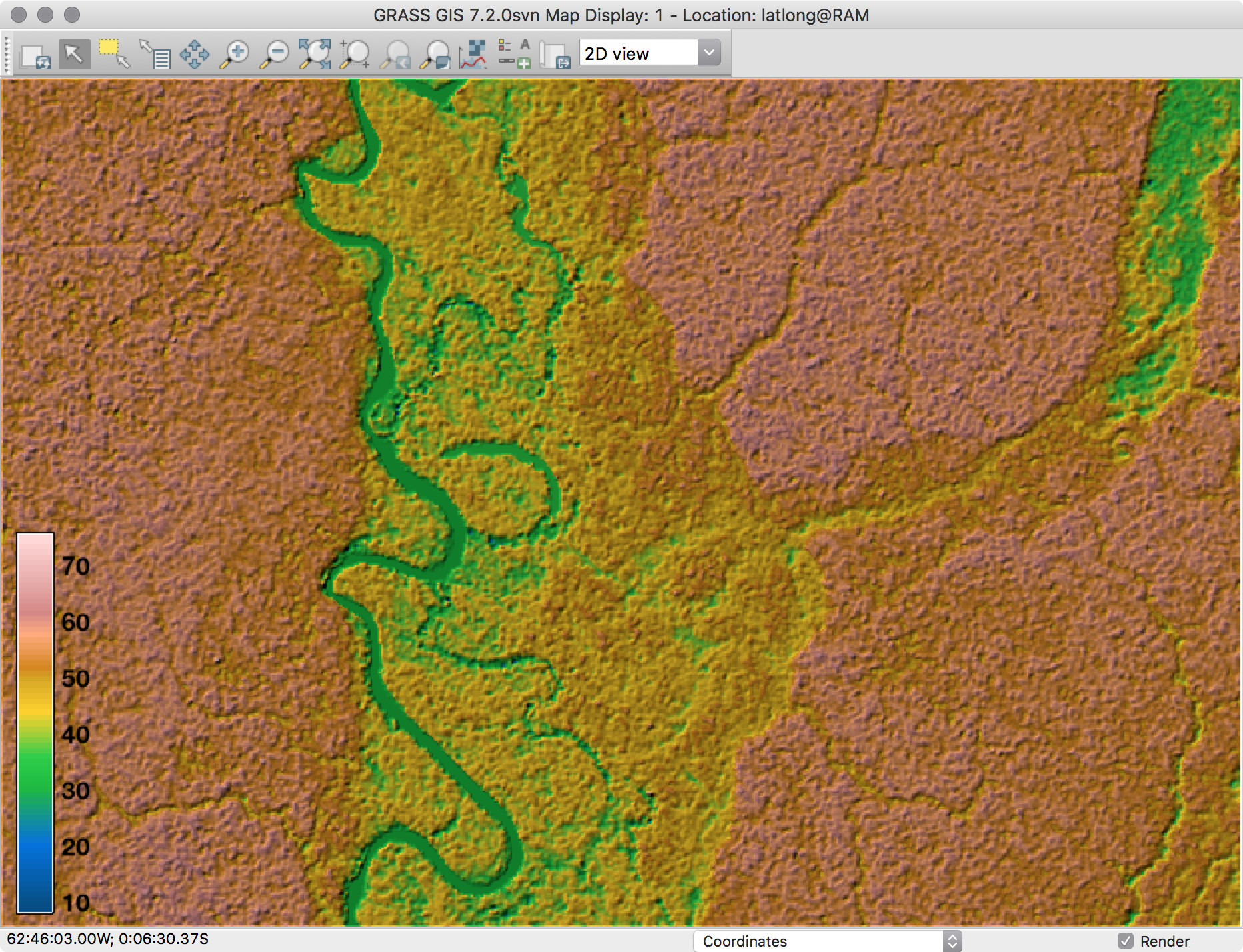
]]>CarlosGrohmannDenoising SRTM with GRASS-GIS2016-12-06T00:00:00-02:002016-12-06T00:00:00-02:00http://carlosgrohmann.com/2016/12/06/denoise-srtm-grassDigital elevation data usually has some noise in it, but removing that noise may not be as easy as a simple filtering procedure. Using raster filters (mean, mode etc) in moving-windows operations will smooth the original topography. One solution is to perform the filtering with the XYZ information of each pixel (that is, treating the DEM as a point cloud and filtering the vector points).
In GRASS-GIS, we can use the r.denoise add-on to do this. The module was originally a bash script that I ported to python (because I needed to call it from a python script, and the bash version wasn’t working this way). The module itself is just a wrapper to the mdenoise (Sun et al., 2007; Stevenson et al., 20109) executable, which needs to be installed and in the system PATH.
To do that, download the source code of mdenoise and compile it:
Now run the module. The mdenoise executable does not work with geographic coordinates, and since I am working on a latitude-longitude location, I need to supply an EPSG code of a projected coordinate system, which will be used for reprojecting the data to a temporary file. In this case I used EPSG=32720, the code for UTM 20S WGS84.
We need to define two parameters, iterations and threshold. From the help page:
The amount of smoothing is controlled by the _threshold_ and _iterations_ parameters. Increasing the _threshold_ decreases how sharp a feature needs to be to be preserved e.g. decreases the smoothing. To preserve ridge crests in mountain areas, T > 0.9 is recommended. Setting T too high results in the preservation of noise. For SRTM data, which is already partly smoothed by NASA, T = 0.99 can be used. Increasing the number of _iterations_ increases the smoothing and the range of spatial correlation of the output dataset. A small number, e.g. 5 or fewer, typically gives the best results.
r.denoise --overwrite input=srtm30m_north output=srtm30m_north_dnoise iterations=5 threshold=0.9 epsg=32720</pre>
Here's the output of the command. For this test area, it took less than 5 seconds to denoise (10 seconds total) on my iMac (4 GHz, 32 GB RAM).
Exporting points...
Projecting...
Denoising...
Input File: tmp_xyz_proj_16395.xyz
Neighbourhood: Common Vertex
Threshold: 0.900000
n1: 5
n2: 50
Read Model...
Triangulation...
0.932 seconds
Denoising Model... 5.151 seconds
Saving Model... 0.186 seconds
Reloading data...
Reading input data...
Writing to output raster map...
r.in.xyz complete. 343865 points found in region.
Removing temporary files...
Removing temporary files...
(Tue Dec 6 11:26:10 2016) Command finished (10 sec)
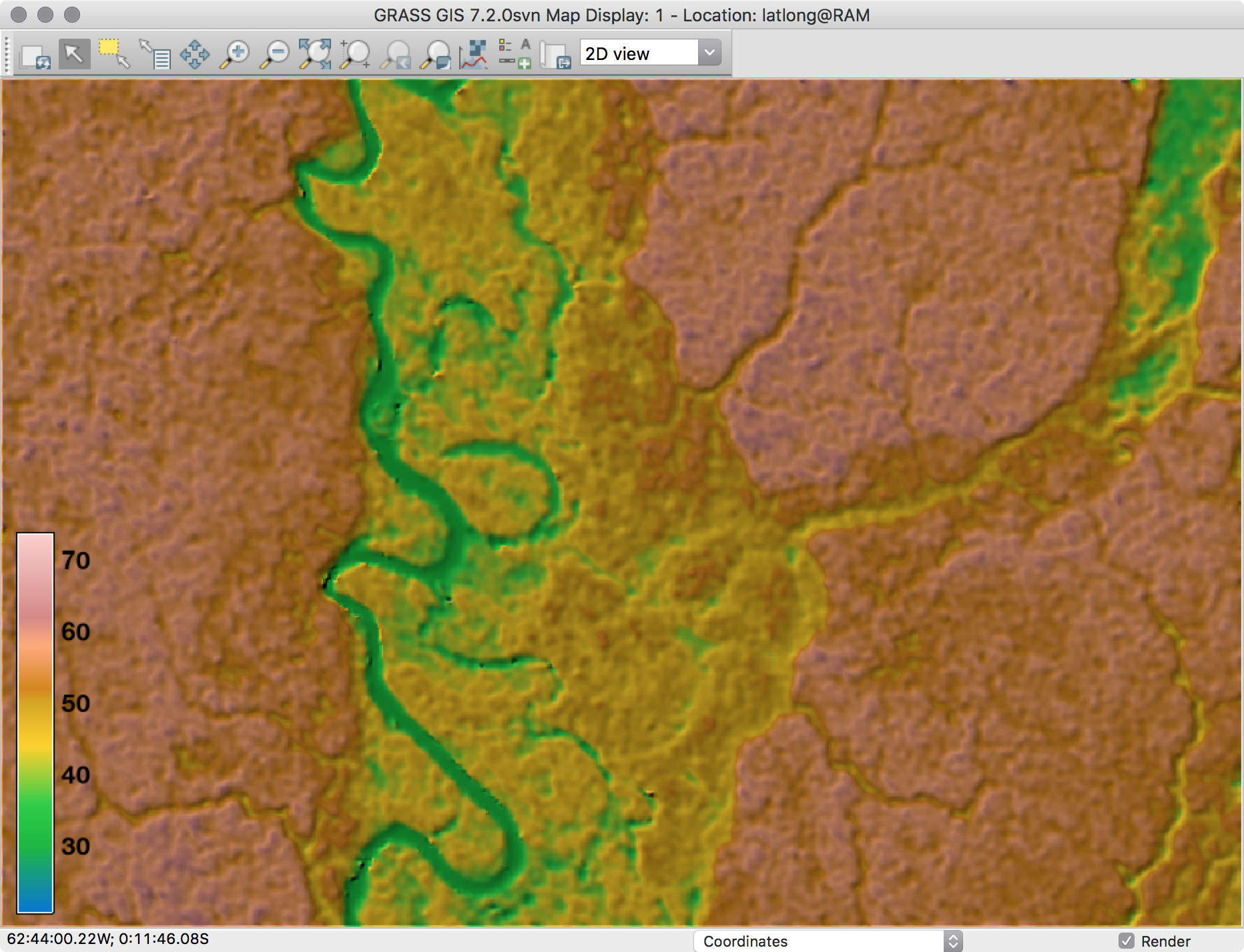
To check the results visually, we can make the same color-shaded composition that we used for the original data:
In GRASS we can use the g.gui.mapswipe module to interactively compares two maps by swiping a visibility bar.
Some quick stats from r.info will show us that the range of elevation values changed a bit:
GRASS 7.2.0svn (latlong):~ > r.info srtm30m_north
 +----------------------------------------------------------------------------+
 | Map:      srtm30m_north                  Date: Wed Jan 14 14:32:07 2015    |
 | Mapset:   RAM                            Login of Creator: guano           |
 | Location: latlong                                                          |
 | DataBase: /Volumes/MacintoshHD2/grassdata                                  |
 | Title:    S01W063.SRTMGL1                                                  |
 | Timestamp: none                                                            |
 |----------------------------------------------------------------------------|
 |                                                                            |
 |   Type of Map:  raster               Number of Categories: 0               |
 |   Data Type:    CELL                                                       |
 |   Rows:         485                                                        |
 |   Columns:      709                                                        |
 |   Total Cells:  343865                                                     |
 |        Projection: Latitude-Longitude                                      |
 |            N:   0:05:53S    S:   0:13:58S   Res: 0:00:01                   |
 |            E:  62:38:53W    W:  62:50:42W   Res: 0:00:01                   |
 |   Range of data:    min = 8  max = 76                                      |
 |                                                                            |
 |   Data Description:                                                        |
 |    generated by r.in.gdal                                                  |
 |                                                                            |
 |   Comments:                                                                |
 |    r.in.gdal input="S01W063.SRTMGL1.bil" output="S01W063.SRTMGL1"          |
 |    r.in.srtm "-1" "input=/Users/guano/Desktop/S01W063.SRTMGL1"             |
 |                                                                            |
 +----------------------------------------------------------------------------+

GRASS 7.2.0svn (latlong):~ > r.info srtm30m_north_dnoise
 +----------------------------------------------------------------------------+
 | Map:      srtm30m_north_dnoise           Date: Tue Dec  6 11:26:09 2016    |
 | Mapset:   RAM                            Login of Creator: guano           |
 | Location: latlong                                                          |
 | DataBase: /Volumes/MacintoshHD2/grassdata                                  |
 | Title:    A denoised version of <srtm30m_north@ram>                        |
 | Timestamp: none                                                            |
 |----------------------------------------------------------------------------|
 |                                                                            |
 |   Type of Map:  raster               Number of Categories: 0               |
 |   Data Type:    FCELL                                                      |
 |   Rows:         485                                                        |
 |   Columns:      709                                                        |
 |   Total Cells:  343865                                                     |
 |        Projection: Latitude-Longitude                                      |
 |            N:   0:05:53S    S:   0:13:58S   Res: 0:00:01                   |
 |            E:  62:38:53W    W:  62:50:42W   Res: 0:00:01                   |
 |   Range of data:    min = 20.5162  max = 73.88921                          |
 |                                                                            |
 |   Data Source:                                                             |
 |    tmp_xyz_merge_16395.xyz                                                 |
 |                                                                            |
 |                                                                            |
 |   Data Description:                                                        |
 |    generated by r.in.xyz                                                   |
 |                                                                            |
 |   Comments:                                                                |
 |    r.in.xyz --overwrite -i input="tmp_xyz_merge_16395.xyz" output="srtm\   |
 |    30m_north_dnoise" method="min" type="FCELL" separator="space" x=1 y=\   |
 |    2 z=3 skip=0 zscale=1.0 value_column=0 vscale=1.0 percent=100           |
 |    Generated by: r.denoise srtm30m_north@RAM iterations=0.9 threshold=5    |
 |                                                                            |
 +----------------------------------------------------------------------------+
</srtm30m_north@ram>
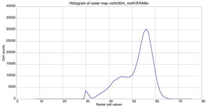
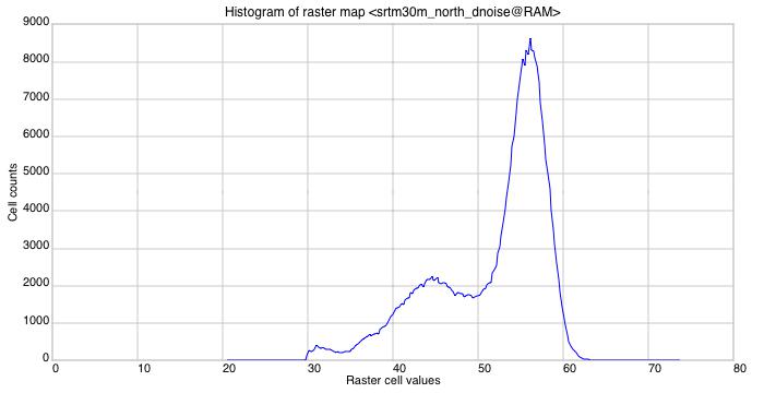
We can also see those changes in the histograms. The curves have the same general shape, but the original data has wider range and larger cell count for the same elevations in the denoised raster.
References
Sun X, Rosin PL, Martin RR, Langbein FC (2007) Fast and Effective Feature-Preserving Mesh Denoising. IEEE Transactions on Visualisation and Computer Graphics, 13(5):925-938 http://dx.doi.org/10.1109/TVCG.2007.1065
]]>CarlosGrohmannCurso Internacional de Espeleoresgate 20162016-05-23T00:00:00-03:002016-05-23T00:00:00-03:00http://carlosgrohmann.com/2016/05/23/curso-internacional-de-espeleoresgate-2016Estão abertas as inscrições para o Curso Internacional de Espeleoresgate 2016.
O curso será realizado na região do Parque Estadual Turístico do Alto Ribeira (PETAR), Vale do Ribeira, São Paulo. Mais precisamente, nas áreas do Bairro da Serra (pertencente ao município de Iporanga) e Núcleos Ouro Grosso e Santana. O Município de Iporanga fica a aproximadamente 300 km de São Paulo, e o Bairro da Serra, a 15 km por estrada de terra da Sede do município. A região representa um das mais importantes regiões cársticas do Brasil com centenas de cavernas cadastradas, trilhas e cachoeiras.
O curso é abrangente com uma ampla programação de aulas práticas. Destinado aos espeleólogos mais experientes e com pleno domínio das técnicas verticais. As atividades têm um apelo prático e abordam os mais modernos e eficientes sistemas de socorro no ambiente cavernícola.
Programação:
Apresentação do curso, instrutores e alunos
Apresentação de históricos e especificidades dos resgates em cavernas na França e Brasil
Técnicas de equipagem de progressão em resgate e regras de segurança
Funções e as competências dos socorristas
Técnicas de assistência à vítima, ponto quente, desobstrução e remoção com maca espeleológica
Apresentação de técnicas e equipamentos de sistemas de comunicação
Organização do resgate e equipes
Gestão do socorro
Exercícios práticos do conteúdo abordado
Simulado final incorporando todo o conteúdo
Datas: de 04 a 11 de setembro de 2016
Os interessados em participar em qualquer um dos módulos devem baixar a FICHA de INSCRIÇÃO, que deve ser enviada com as informações solicitadas para o email eziorubbioli@gmail.com até o dia 30 de junho. A comissão organizadora irá avaliar o perfil e experiência dos candidatos confirmando a reserva até o dia 15 de julho.
A partir da confirmação, os interessados terão um prazo de 10 dias para efetuar o pagamento. Lembramos que o não cumprimento deste prazo implica no cancelamento imediato da inscrição. O número de vagas é limitado e existe um grande número de interessados.
Prazos:
Até 30 de junho: envio da ficha de pré-inscrição De 01 a 15 de julho: confirmação e aceitação da inscrição Dia 29 de julho: data limite do pagamento da primeira parcela. Dia 15 de agosto: pagamento final Mais informações estão disponíveis na Primeira Circular.
Comments
Deyvid Santana: Esterei pronto e em condiçõesw mais uma vez com essa galera.