resample and derive or derive and resample? [paper review]

Working with Digital Elevation Models (DEMs) have became a standard practice in scientific disciplines related to the physical environment, from geomorphology, geology, to biogeography and climate modeling. The Shuttle Radar Topography Mission (SRTM - Farr et al., 2007) and ASTER GDEM (Tachikawa et al., 2011) provide a near-global to global coverage at medium spatial resolution (30 to 90m) free of charge, while WorldDEM (Krieger et al., 2009) is a global dataset with 12m resolution and ALOS World3D (Tadono et al., 2014) delivers a global DEM with only 5m resolution.

The only problem with these data is when we need to make some analysis in a regional scale. By ‘regional’ I mean very very large. Like the entire Amazon Basin, or even the whole world. One common option is to use DEMs with coarser resolution like SRTM30_PLUS (Becker et al., 2009) with a resolution of 30’’ (about 1 km) or ETOPO1 (Amante and Eakins, 2009) with 1’ resolution. But if you are working with any geomorphometric parameter like slope (or gradient), aspect, roughness, etc, you might ask yourself if using a coarser DEM is your best option. These 1km DEMs are generated by averaging the higher resolution data with moving-window filters, and that is a process known to cause smoothing of the topographical surface (see Carter, 1992; Zhang and Montgomery, 1994; Grohmann and Riccomini, 2009).

At this point you are facing two choices:

• Derive your geomorphometric data from a higher resolution DEM and then resample it to a coarser resolution for the regional analysis;
  or
• Resample the higher resolution DEM into a coarser one and derive the geomorphometric data from this coarse DEM (which would be the same as deriving the parameters from SRTM30_PLUS, for example)

So I decided to test these two scenarios, and the results are published in this article:

Grohmann, C. H., 2015. Effects of spatial resolution on slope and aspect derivation for regional-scale analysis. Computers & Geosciences 77, pp. 111–117. http://dx.doi.org/10.1016/j.cageo.2015.02.003

(if you want to read it and find yourself behind Elsevier’s paywall, you can grab the PDF of the uncorrected proof at the Publications section of this website)

All the analysis were run within GRASS-GIS using Python scripts and the pyGRASS library to access GRASS’ datasets. Numerical analysis were done with Scipy, Numpy and the R package circular. Plots were created with Matplotlib and final figures were created on Inkscape. Following those questions we asked earlier, the analysis was done in two parts:

1. Parameters derived from a resampled DEM: in this case, an original DEM with 03’’ resolution (about 90m) was resampled by averaging the pixel values in cell of 0.3km, 0.45km, 0.6km, 0.75km, 0.9km, 1.05km, 1.2km, 1.4km, 1.55km and 1.85km. For each resampled DEM, slope and aspect were calculated using GRASS tools.

2. Resampled parameters from a base DEM: here, I calculated slope and aspect for the original 03’’ DEM and then resampled them to the same spatial resolutions as in the previous case. Resampled slope was considered as the average of values in the new pixel, while resampled aspect was calculated as the vectorial mean of the values.

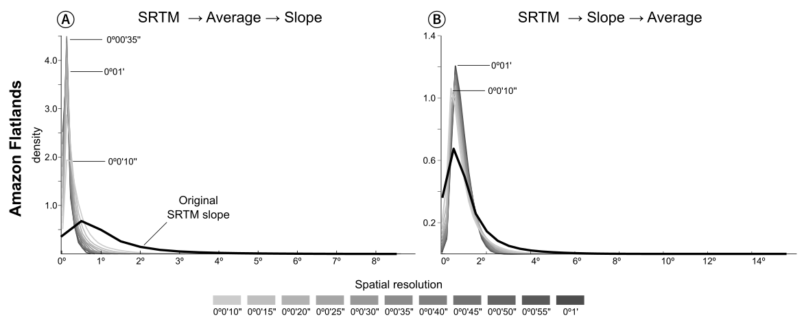
The figures below show some of the results for the Amazon basin (flat landscape): Averaging the DEM prior to calculating the derivatives (fig.A) will smooth the topographical surface, so the calculated slopes will be much smaller than those calculated from the original DEM. See how the density curve becomes way more asymmetrical with resampling. Calculating the derivatives from the higher resolution data and then resampling will result in less change to the slope values.

Aspect is less sensitive to the resampling approaches used in this study, but the peaks and valleys of the density plot become more pronounced as resolution decreases. The original curves are flatter, so the aspect values are more evenly distributed, without any significant tendency for a preferred orientation.

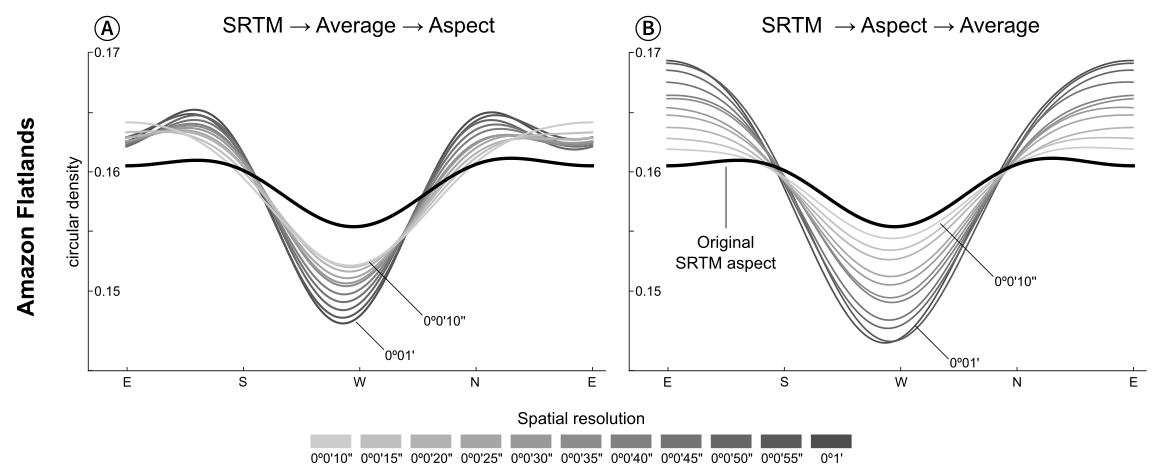
The take-away message here is that you should always try to calculate surface parameters (such as aspect and slope) from a higher resolution DEM, and in case needed, resample them to a coarser resolution. Sometimes this may seem counter-productive, because it might take a long time to process the higher resolution DEMs, but the end results are worthwhile. The results for two other test areas (one in a hilly region in southeastern Brazil and another in the Andes Mountains) are in the paper. Give it a try and leave any comments below.    

Note:  The images from the article were reused with permission from Elsevier.

References [Amante and Eakins, 2009] Amante, C. and Eakins, B. W., 2009. ETOPO1 1 Arc-Minute Global Relief Model: Procedures, Data Sources and Analysis. Technical report, NOAA Technical Memorandum NES- DIS NGDC-24. 19 pp.

[Becker et al., 2009] Becker, J.J., Sandwell, D.T., Smith, W.H.F., Braud, J., Binder, B., Depner, J., Fabre, D., Factor, J., Ingalls, S., Kim, S.H., Ladner, R., Marks, K., Nelson, S., Pharaoh, A., Trimmer, R., von Rosenberg, J., Wallace, G., Weatherall, P., 2009. Global bathymetry and elevation data at 30 arcseconds resolution: SRTM30_PLUS. Marine Geodesy 32, 355–371.

[Carter, 1992] Carter, J. R., 1992. The Effect Of Data Precision On The Calculation Of Slope And Aspect Using Gridded Dems. Cartographica: The International Journal for Geographic Information and Geovisualization 29, pp. 22–34.

[Farr et al., 2007] Farr, T.G., Rosen, P.A., Caro, E., Crippen, R., Duren, R., Hensley, S., Kobrick, M., Paller, M., Rodriguez, E., Roth, L., Seal, D., Shaffer, S., Shimada, J., Umland, J., Werner, M., Oskin, M., Burbank, D., Alsdorf, D., 2007. The shuttle Radar topography mission. Rev. Geophys. 45, RG2004.

[Grohmann and Riccomini, 2009] Grohmann, C.H., Riccomini, C., 2009. Comparison of roving-window and search-window techniques for characterising landscape morphometry. Computers & Geosciences 35, 2164–2169.

[Krieger et al., 2009] Krieger, G., Zink, M., Fiedler, H., Hajnsek, I., Younis, M., Huber, S., Bachmann, M., Gonzalez, J., Schulze, D., Boer, J., Werner, M., Moreira, A., 2009. The TanDEM-X Mission: overview and status. In: Radar Conference, 2009, IEEE, California, USA, pp. 1–5.

[Tachikawa et al., 2011] Tachikawa, T., Hato, M., Kaku, M. and Iwasaki, A., 2011. Characteristics of ASTER GDEM version 2. In: Geoscience and Remote Sensing Symposium (IGARSS), 2011 IEEE Interna- tional, pp. 3657–3660.

[Tadono et al., 2014] Tadono, T., Ishida, H., Oda, F., Naito, S., Minakawa, K. and Iwamoto, H., 2014. Precise Global DEM Generation by ALOS PRISM. ISPRS Annals of Photogrammetry, Remote Sensing and Spatial Information Sciences II-4, pp. 71–76.

[Tadono et al., 2014] Zhang, W. and Montgomery, D., 1994. Digital elevation model grid size, landscape representation, and hydrologic simulations. Water Resources Research 30(4), pp. 1019–1028.